Ray tracing. What a word. Tears, both of joy and desperation. Deubgging for hours to find that you were using floats instead of doubles 3 parts ago. What a trip. Here we traced a ray along the entire pipeline. We started out by determining when it intersects with different objects in our scene. Then, we made it hella faster by using the slickest of the data structres, the BVH. Now that things were running at a sane speed, we decided to make the lighting more realilistic by modeling the light coming from the sources as either uniformly eminating in the hemisphere surrounding the light, or by implementing a slick monte carlo estimation of the light. Next, we took that light model and let the rays bounce around more than once so we could get more accurately model the infinite potential bounces of a normal ray of light. Finally, we optimized our pixel sampling so we don't have to wait days to get a 2048 sampled image to render.
Part 1: Intersect
Ray generation
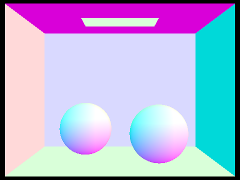
We generate rays by pretending a ray is going from the pixel to the light source. This is so we don't waste time chasing rays that don't hit anything in the secen. We geometrically create rays by specifying an origin and a direction and we find intersections based on the shape of the primitive in the scene. Primitives are just basic shapes that are used to create the scene. For example, the CBspheres one, is five rectangles aranged in a box, with an additional rectangle as a window and two spheres showing prominently inside the box.
Triangle Intersection
With some hefty help from the slides, I implemented triangle intersection, with the Moller Trumbore Algorithm. It calculates the time of intersection and the barycentric coordinates of the intersection point. What the algorithm really does is find how many direction vectors we need to line up for the ray to intersect the triangle. Next, it finds the barycentric coordinates of the point, so we can check the sign and see if it actually intersects. We determine this by checking if the time is within tmin, tmax and if all of the barycentric coordinates are positive.
Sphere Intersection
With some hefty help from a different set of slides, I implemented sphere intersection, with a modified quadratic formula. We essentially just found the solutions to the quadratic and checked if they were valid intersection points.
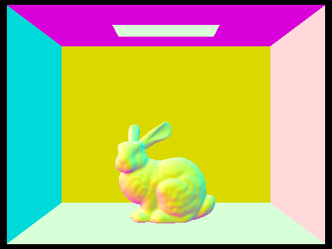
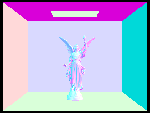
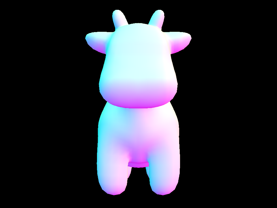
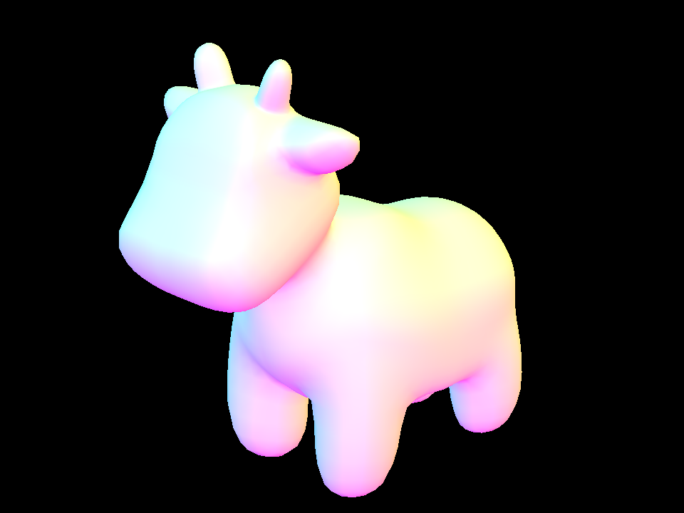
Normal shading examples
|
|
|
Part 2: BVH
Construction
We construct our BVH by first constructing a bbox that encompasses all of the primitives in our scene. Then we sort the objects and sort them so we can split them in the middle. This makes each branch have half of the objects ensuring that the tree is of minimum depth. Therefore the binary searching through the tree takes the minimal amount of time. Then we recursively construct a BVH node until the size of the array of primitives is less than or equal to our max_leaf size.
Intersection
For intersection, I compute the max value for each dimension for the bbox, subtract the origin and divide by the direction of the ray. I then take the max of the minimum values and the min of the maxium values to get the min and max respectively. These form an interval for where the ray intersect with the bbox.
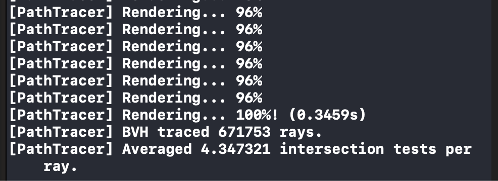
Here's some example output that shows the difference in number of required intersection tests before and after implementing the BVH.

|
|
Analysis
The BVH functions very similarly to a binary tree asymptotically. At each split, you get to ignore approximately half of the primitives. You then recursively split until you hit a leaf_node. You will execute approximately ` log(num_primitives / max_leaf_size) ` splits before running intersection tests on at most ` max_leaf_size ` primitives per leaf node that the ray hits, so for ` max_leaf_size = 4 ` and ` num_primitives = 1000 ` we will perform 8 splits and run 4 intersection tests per BVH_leaf_node that the ray hits. If we did not use the acceleration, we would try to intersect the ray with every primitive in the scene making us perform 1000*num_rays tests as opposed to num_rays*(num_primitives in leaf node bbox that intersect) and ` num_primitives in leaf node bbox that intersect ` is generally much lower than the num_primitives. In the example above, we see that implementing the BVH sped up our render time for the cow 140 times. We averaged .3% of the required ray intersection tests.
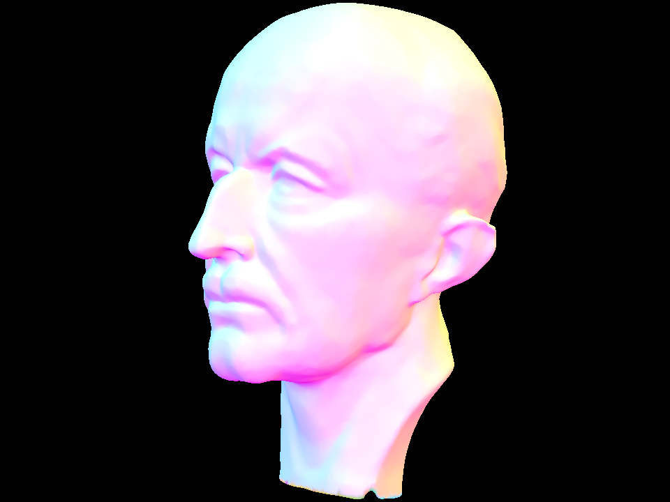
Here's some of the more complicated scenes that would've taken me forever to render without the blessed BVH.
|

|
|
|
Part 3: Direct illumination
A tale of two light sources
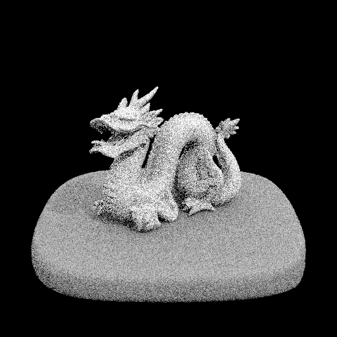
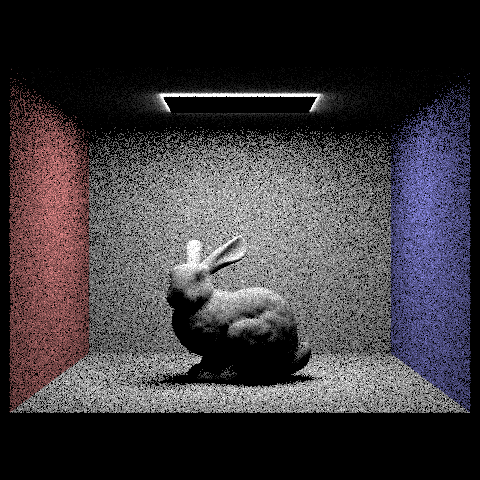
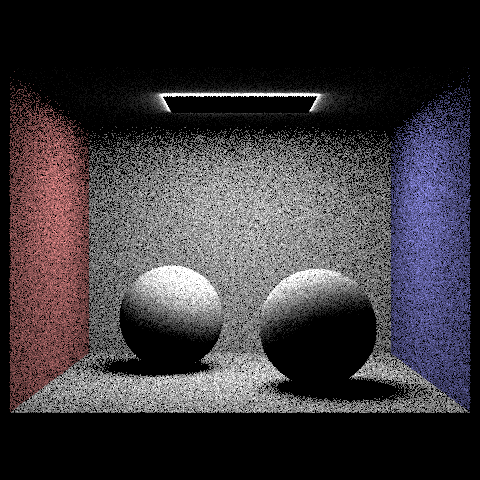
Hemisphere light sampling generates a light ray by sampling uniformly at random from the entire hemisphere eminating from the light source. For this method, we essentially just generate num_sample number of rays and check if they intersect the bvh. If it does, we factor in it's contribution to the color using the bsdf of the surface it hit and some other mathy factors to average everything in correctly. For Importance sampling, we think of drawing rays from our point to different locations on the light source. We can think of them as shadow rays if they intersect something in the scene, because then the light from the source is blocked. We proceed pretty similarly to the previous part except this time we only factor in the color if there are not intersections, ie. there's a path from the point to the light. This is a more efficient method as we know our ray has the potential to hit the light source. Look at the next section for more details.
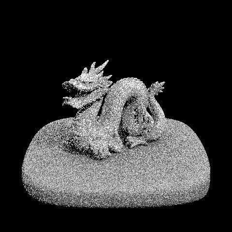
One scene with all the options
Notice how the noise levels in soft shadows decrease so sharply between one and sixteen
|
|
|

|
Some results of Hemisphere
|
|
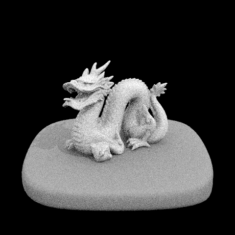
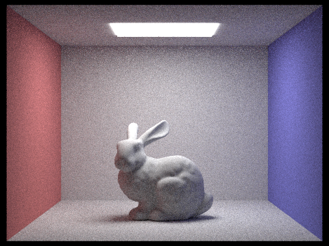
Some results of Importance
|

|
Hemisphere vs light sampling Analysis
As I was getting into above, hemisphere sampling is much noisier at the same sample rate because each sample does less work. The importance sampling uses the power of good ole monte carlo to make our samples count for more and have more denoising power. The randomness of hemispheric sampling is actually to it's disservice as it cannot take advantage of the very different relative importance of different potential samples.
Part 4: Global illumination
How'd we do it
So, what we did here was take a ray. If our depth is zero we just return the color of it if it's a light source. If our depths is bigger, then things get interesting. For a depth of one, we just kinda check if we intersect with anything and return it's color if we do. Sounds awfully familiar ha? That's cause we did it in part 3 so we just call that. Now is the juicy part, if our depth is greater than one, we want to get the indirect lighting on the point. So we just keep bouncing the ray until we hit our max_depth or russian roullete terminates it. There was a lotta nitty gritty details, but that's the main idea:)
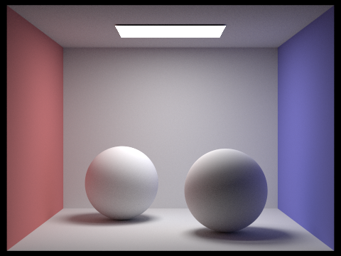
Some global 1024s
Notice how the indirect and direct illumination interplay. We can see the colors from the walls on parts of the spheres because of the indirect illumination. WILD

|
|
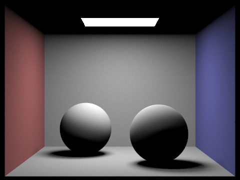
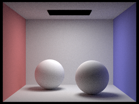
Direct vs indirect
Notice what happens to the light source. When we only have direct illumination, we only really see what is one bounce away. When we take that out for indirect illumination, we can't see the light anymore.
|
|
CBunny dae!
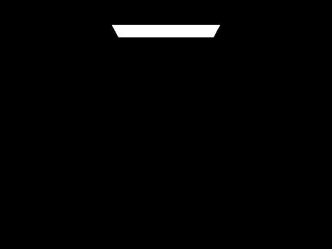
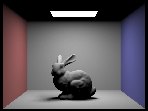
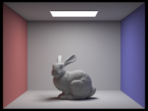
Notice what happens to the light source at really low depths. It is the only thing showing! Why is that? Because at depth 0, we can only check if we are a light source or not. WHy's the roof gone for depth 1? Because nothing can make it back to the roof within one bounce. The middle ones don't seem to surprising, as you increase the depth, more surfaces become eligible to be illuminated. But why is 100 not super overexposed?? Russian roullete to the rescue! Because of Russian roullete we can depend on rays terminating before they can infect every surface, more precisely, the rays terminate within a couple of steps, likely fewer than 10.
|
|
|

|

|

|
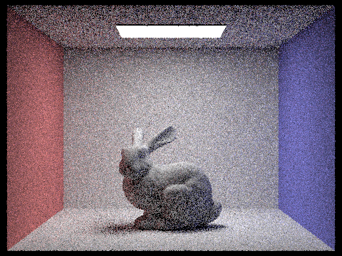
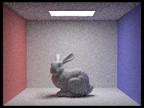
CBunny dae 2!
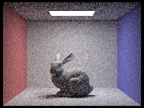
Notice the power of da sample at reducing noise!
|
|
|

|

|

|

|
Part 5: Adaptive sampling
How'd we adapt
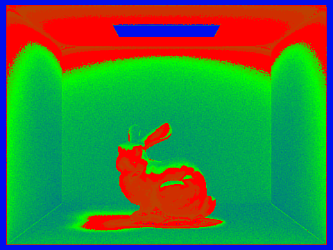
I followed the formula given in the slides with some slick modifications. We learned in class that division is the real slowdown, so I tried to move as much division I could out of my loops by calculating reciprocals once, then just using them. Besides that, I implemented the magic_eye test, my name for the I value we get from that 1.96 confidence interval value, and we got some cool results. Check em out:)
Adaptive sampling example

|
|